Annotation
1. Genomic Element Distribution Analysis
This workflow provides two complementary ways to perform genomic distribution analysis across multiple annotation layers. Users may either run a single wrapper function to execute all selected analyses in one step, or call each annotation function individually for inspection of intermediate results.
Integrated workflow (recommended):
Thegenomic_distribution()wrapper function executes one or more distribution analyses within a single, unified pipeline. According to the specifieddistributionsargument, it internally invokes the four distribution functions in sequence, while automatically handling shared parameters and organizing all outputs in a common directory.Step-by-step workflow:
The individual functionsgenic_distribution(),ccre_distribution(),chromhmm_distribution(), andrepeat_distribution()can be run independently. This approach allows users to customize parameters for each analysis and to inspect intermediate results with greater flexibility.
Wrapper Function Overview
The genomic_distribution() function performs genomic
distribution analyses across multiple annotation types.
Parameters
| Parameter | Type | Default | Description | Example |
|---|---|---|---|---|
query
|
GRanges or GRangesList | — |
Genomic regions to be annotated. When a GRangesList is
provided, each element is treated as an independent sample or cluster.
|
query = my_peaks
|
out_dir
|
character | — | Output directory used to store all result tables and plots. The directory is created automatically if it does not exist. |
out_dir = “./distribution_results”
|
distributions
|
character |
c(“genic”, “ccre”)
|
Annotation layers to run. Supported options include
“genic”, “ccre”, “chromhmm”, and
“repeat”. Multiple annotation layers can be selected
simultaneously.
|
distributions = c(“genic”, “repeat”)
|
ref_genome
|
character |
“hg38”
|
Reference genome version used for annotation. Supported options are
“hg38” and “mm10”.
|
ref_genome = “mm10”
|
ref_source
|
character |
“knownGene”
|
Gene annotation source used for genic annotation.
“knownGene” uses UCSC knownGene annotations via TxDb
packages, while “GENCODE” uses reference annotations from
GENCODE (Release 49 for hg38 and vM35 for mm10).
|
ref_source = “GENCODE”
|
mode
|
character |
“nearest”
|
Assignment mode for overlapping features. “nearest” assigns
each query region to the closest feature, while “weighted”
assigns features proportionally based on overlap length.
|
mode = “weighted”
|
plot
|
logical |
TRUE
|
Whether to generate stacked bar plots in addition to summary tables. |
plot = FALSE
|
Example Usage
library(multiEpiCore)

genomic_distribution(
  query = my_grl,
  out_dir = "./genomic_distribution_results",
  distributions = c("genic", "ccre", "chromhmm", "repeat"),
  ref_genome = "hg38",
  ref_source = "knownGene",
  mode = "nearest",
  plot = TRUE
)
1A. Genic Distribution Analysis
The genic_distribution() function annotates genomic
regions with gene structural features, calculates
overlap-based feature proportions, and generates a summary table with an
optional visualization. The genic categories are defined as follows:
- Promoter: Regions defined as the 1,000 bp upstream of transcription start sites (TSS), representing promoter-proximal regulatory sequences associated with transcription initiation.
- 5’ UTR: Untranslated regions at the 5’ end of
transcripts.
- Exon: Exonic regions corresponding to coding sequences only. Since untranslated regions are excluded, this category represents protein-coding portions of transcripts.
- Intron: Non-coding regions spliced out during
transcript processing, often enriched for regulatory elements.
- 3’ UTR: Untranslated regions at the 3’ end of transcripts.
Parameters
| Parameter | Type | Default | Description | Example |
|---|---|---|---|---|
query
|
GRangesList or GRanges | — | Query regions to be annotated with gene structure features. |
query = my_peaks
|
out_dir
|
character |
“./”
|
Output directory used to store annotation results. The directory is created automatically if it does not exist. |
out_dir = “./genic_results”
|
ref_genome
|
character |
“hg38”
|
Reference genome version. Supported options are “hg38” and
“mm10”.
|
ref_genome = “mm10”
|
ref_source
|
character |
“knownGene”
|
Gene annotation source used to define gene models.
“knownGene” uses UCSC manually curated gene models via TxDb
packages, while “GENCODE” uses comprehensive reference
annotations from GENCODE (Release 49 for hg38 and vM35 for mm10).
|
ref_source = “GENCODE”
|
mode
|
character |
“nearest”
|
Annotation assignment mode. “nearest” assigns each region
to the closest gene feature, while “weighted” assigns
features proportionally based on overlap length.
|
mode = “weighted”
|
plot
|
logical |
TRUE
|
Whether to generate a stacked barplot showing the distribution of genic features. |
plot = FALSE
|
Output Files
The function generates the following output files in the specified
out_dir:
- cCRE annotation table -
genic_distribution.tsv- Tab-delimited table of genic category percentages
- Rows: samples/clusters from input
- Columns: genic categories
- Values: percentage of each category class per sample/cluster
- cCRE distribution plot -
genic_distribution.pdf(ifplot = TRUE)- Stacked bar plot showing genic composition across samples or clusters
- X-axis: percentage (0-100%)
- Y-axis: samples/clusters
1B. cCRE Distribution Analysis
The ccre_distribution() function annotates genomic
regions with candidate cis-regulatory elements (cCREs)
using RepeatMasker data, calculates overlap-based repeat class
proportions, and outputs a summary table with an optional visualization.
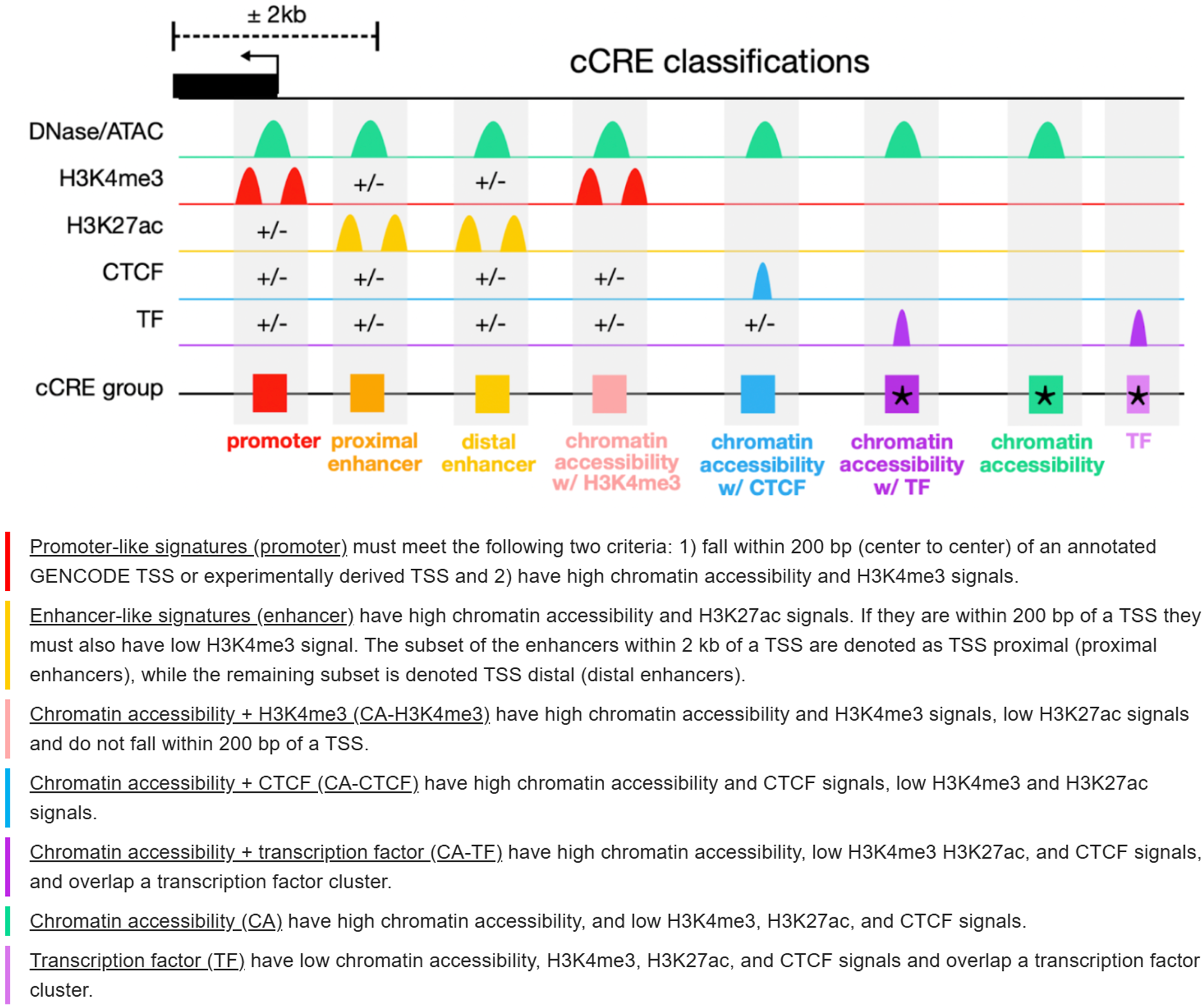
The cCRE categories are defined as follows:
Promoter (Promoter-like signature):
cCREs located within 200 bp of an annotated or experimentally supported TSS. They show high chromatin accessibility together with strong H3K4me3 enrichment, consistent with active transcription initiation sites.Enhancer (Enhancer-like signature):
cCREs with high chromatin accessibility and strong H3K27ac signals. Elements within 2 kb of a TSS are classified as TSS-proximal enhancers, while those farther away are classified as TSS-distal enhancers. Regions within 200 bp of a TSS must have low H3K4me3 to avoid promoter assignment.CA-H3K4me3 (Chromatin accessibility with H3K4me3):
cCREs showing high chromatin accessibility and H3K4me3 enrichment, low H3K27ac, and located outside the 200 bp TSS window. These regions resemble promoter-like chromatin states but are not directly associated with annotated TSSs.CA-CTCF (Chromatin accessibility with CTCF):
cCREs characterized by high chromatin accessibility and CTCF binding, with low H3K4me3 and H3K27ac signals. They are typically associated with chromatin insulation and higher-order genome organization.CA-TF (Chromatin accessibility with transcription factor binding):
cCREs with high chromatin accessibility that overlap transcription factor binding clusters, while showing low H3K4me3, H3K27ac, and CTCF signals. These regions likely represent TF-driven regulatory sites.CA (Chromatin accessibility only):
cCREs marked by high chromatin accessibility but lacking H3K4me3, H3K27ac, and CTCF signals. They may represent open chromatin regions with potential or context-dependent regulatory activity.TF (Transcription factor binding):
cCREs overlapping transcription factor binding clusters but showing low chromatin accessibility and low levels of H3K4me3, H3K27ac, and CTCF signals. These sites may reflect transient or condition-specific TF occupancy.
Parameters
| Parameter | Type | Default | Description | Example |
|---|---|---|---|---|
query
|
GRangesList or GRanges | — | Query regions to be annotated with cCRE elements. |
query = my_peaks
|
out_dir
|
character |
“./”
|
Output directory used to store annotation results. The directory is created automatically if it does not exist. |
out_dir = “./ccre_results”
|
ref_genome
|
character |
“hg38”
|
Reference genome version. Supported options are “hg38” and
“mm10”.
|
ref_genome = “mm10”
|
mode
|
character |
“nearest”
|
Annotation assignment mode. “nearest” assigns each region
to the closest cCRE category, while “weighted” assigns
categories proportionally based on overlap length.
|
mode = “weighted”
|
plot
|
logical |
TRUE
|
Whether to generate a stacked barplot showing the distribution of cCRE categories. |
plot = FALSE
|
Output Files
The function generates the following output files in the specified
out_dir:
- cCRE annotation table -
ccre_distribution.tsv- Tab-delimited table of cCRE category percentages
- Rows: samples/clusters from input
- Columns: cCRE categories
- Values: percentage of each category class per sample/cluster
- cCRE distribution plot -
ccre_distribution.pdf(ifplot = TRUE)- Stacked bar plot showing cCRE composition across samples or clusters
- X-axis: percentage (0-100%)
- Y-axis: samples/clusters
1C. ChromHMM Distribution Analysis
The chromhmm_distribution() function annotates genomic
regions with chromatin states using ChromHMM data,
calculates overlap-based chromatin state proportions, and produces a
summary table with an optional visualization.
Acet: Acetylation-associated active regulatory regions
EnhWk: Weak enhancers
EnhA: Active enhancers
PromF: Promoter flanking regions
TSS: Transcription start sites
TxWk: Weak transcription
TxEx: Transcription with exon signals
Tx: Transcription
OpenC: Open chromatin
TxEnh: Transcribed enhancers
ReprPCopenC: Polycomb-repressed regions with open chromatin
BivProm: Bivalent promoters
ZNF: Zinc finger gene clusters
ReprPC: Polycomb-repressed chromatin
HET: Constitutive heterochromatin
GapArtf: Assembly gaps and artifacts
Quies: Quiescent background
Parameters
| Parameter | Type | Default | Description | Example |
|---|---|---|---|---|
query
|
GRangesList or GRanges | — | Query regions to be annotated with cCRE elements. |
query = my_peaks
|
out_dir
|
character |
“./”
|
Output directory used to store annotation results. The directory is created automatically if it does not exist. |
out_dir = “./ccre_results”
|
ref_genome
|
character |
“hg38”
|
Reference genome version. Supported options are “hg38” and
“mm10”.
|
ref_genome = “mm10”
|
mode
|
character |
“nearest”
|
Annotation assignment mode. “nearest” assigns each region
to the closest cCRE category, while “weighted” assigns
categories proportionally based on overlap length.
|
mode = “weighted”
|
plot
|
logical |
TRUE
|
Whether to generate a stacked barplot showing the distribution of cCRE categories. |
plot = FALSE
|
Output Files
The function generates the following output files in the specified
out_dir:
- ChromHMM annotation table -
chromhmm_distribution.tsv- Tab-delimited table of ChromHMM state percentages
- Rows: samples/clusters from input
- Columns: cCRE categories
- Values: percentage of each category class per sample/cluster
- ChromHMM distribution plot -
chromhmm_distribution.pdf(ifplot = TRUE)- Stacked bar plot showing repeat class composition across samples or clusters
- X-axis: percentage (0-100%)
- Y-axis: samples/clusters
1D. Repeat Distribution Analysis
The repeat_distribution() function anotates genomic
regions with chromatin states using ChromHMM data, computes
overlap-based chromatin state percentages, and generates a summary table
along with an optional visualization.
SINE: Short interspersed nuclear elements
LINE: Long interspersed nuclear elements
LTR: Long terminal repeat retrotransposons
Retroposon: Non-LTR retrotransposon-derived elements
RC: Rolling-circle transposons
DNA: DNA transposons
Satellite: Satellite repeats
Simple_repeat: Simple sequence repeats
Low_complexity: Low-complexity sequences
rRNA: Ribosomal RNA repeats
tRNA: Transfer RNA repeats
snRNA: Small nuclear RNA repeats
scRNA: Small cytoplasmic RNA repeats
srpRNA: Signal recognition particle RNA repeats
RNA: Other RNA-related repeats
Unknown: Unclassified repeat elements
Parameters
| Parameter | Type | Default | Description | Example |
|---|---|---|---|---|
query
|
GRangesList or GRanges | — | Query regions to be annotated with cCRE elements. |
query = my_peaks
|
out_dir
|
character |
“./”
|
Output directory used to store annotation results. The directory is created automatically if it does not exist. |
out_dir = “./ccre_results”
|
ref_genome
|
character |
“hg38”
|
Reference genome version. Supported options are “hg38” and
“mm10”.
|
ref_genome = “mm10”
|
mode
|
character |
“nearest”
|
Annotation assignment mode. “nearest” assigns each region
to the closest cCRE category, while “weighted” assigns
categories proportionally based on overlap length.
|
mode = “weighted”
|
plot
|
logical |
TRUE
|
Whether to generate a stacked barplot showing the distribution of cCRE categories. |
plot = FALSE
|
Output Files
The function generates the following output files in the specified
out_dir:
- Repeat annotation table -
repeat_distribution.tsv- Tab-delimited table of repeat class percentages
- Rows: samples/clusters from input GRangesList
- Columns: repeat element categories ordered as:
- Transposable elements: SINE, LINE, LTR, Retroposon, RC, DNA
- Structural variants: Satellite, Simple_repeat, Low_complexity
- RNA genes: rRNA, tRNA, snRNA, scRNA, srpRNA, RNA
- Unknown
- Values: percentage of each repeat class per sample
- Repeat distribution plot -
repeat_distribution.pdf(ifplot = TRUE)- Stacked barplot visualization
- X-axis: percentage (0-100%)
- Y-axis: samples/clusters (reversed order)
- Colors: Dark2 palette from RColorBrewer
- Dimensions: 6 inches (width) × 5 inches (height)
- Features: Minimal theme with horizontal legend at right
2. TFBS Enrichment Analysis
2A. Generate matched control regions
The get_matched_control() function generates background
control regions by randomly selecting genes with similar length to the
nearest gene of each query region, then placing control regions at the
same TSS-relative distance on the selected genes. This approach
preserves the relationship between peaks and gene structure while
avoiding biases from using the same genomic neighborhoods.
What this function does:
For each query genomic region: - Identify the nearest gene (used only to define the TSS-relative offset) - Compute the signed distance to the gene TSS, accounting for strand
To generate control regions: - Select genes with similar lengths (excluding the original gene) - Randomly sample matched genes as anchors - Place control regions at the same TSS-relative positions
Quality control: - Automatically relax gene length tolerance if candidates are insufficient - Discard control regions outside valid chromosome boundaries
Output: - Generate multiple control regions per query region (configurable replicates) - Return all control regions as a single GRanges object
Parameters
| Parameter | Type | Default | Description | Example |
|---|---|---|---|---|
query
|
GRanges or GRangesList | — |
Query regions used for control region generation. When a
GRangesList is provided, control regions are generated
separately for each element and then combined.
|
query = my_peaksquery = peak_clusters
|
ref_genome
|
character |
“hg38”
|
Reference genome version. Supported options are “hg38”
(Human GRCh38) and “mm10” (Mouse GRCm38).
|
ref_genome = “hg38”
|
ref_source
|
character |
“knownGene”
|
Gene annotation source used for defining gene models.
“knownGene” uses UCSC TxDb annotations, while
“GENCODE” uses GENCODE reference annotations (v49 for hg38
and vM23 for mm10).
|
ref_source = “GENCODE”
|
style
|
character |
NULL
|
Chromosome naming style. If NULL, the naming style is
automatically inferred from the input query object.
|
style = “UCSC”
|
n_rep
|
integer |
1
|
Number of control regions generated per query region. |
n_rep = 3
|
regions
|
integer |
800
|
Width of control regions in base pairs, centered on the calculated genomic position. |
regions = 500
|
seed
|
integer |
42
|
Random seed used to ensure reproducible control region selection. |
seed = 12345
|
length_tolerance
|
numeric |
0.2
|
Initial tolerance for gene length matching. A value of 0.2
corresponds to ±20% tolerance. If insufficient candidates are found, the
tolerance is automatically relaxed up to ±100%.
|
length_tolerance = 0.3
|
- Input flexibility:
- Accepts GRanges: Single set of peaks (e.g., all CTCF binding sites)
- Accepts GRangesList: Multiple peak sets (e.g., biclustering results with named clusters)
- For GRangesList, controls are generated per element, then merged into single GRanges output
- Gene annotation sources:
- knownGene: UCSC knownGene (TxDb), conservative and widely used
- GENCODE: Filtered GENCODE annotations
- Only genes with supported transcript evidence are retained
- Control region generation:
- For each query peak, the nearest gene is first identified and used only as an anchor to define the signed distance between the peak center and the gene TSS.
- A set of matched genes is then selected based on gene length
similarity, with an initial tolerance of ±
length_tolerancethat is adaptively relaxed up to ±100% if needed. - Control regions are generated by placing regions at the same TSS-relative distance on the matched genes.
- Only standard autosomes and sex chromosomes are used (hg38: chr1–chr22, chrX, chrY; mm10: chr1–chr19, chrX, chrY), and any control regions falling outside valid chromosome boundaries are discarded.
Output
The function returns a GRanges object containing all successfully generated control regions.
Object type: GRanges (GenomicRanges package)
Number of regions:
- For GRanges input: Up to
n_rep × length(query)regions - For GRangesList input: Up to
n_rep × sum(lengths(query))regions - Actual count may be lower if some controls fail boundary validation
- Each query peak ideally generates
n_repcontrol regions
- For GRanges input: Up to
Region characteristics:
- Width: All regions have uniform width specified by
regionsparameter - Positioning: Centered on calculated TSS-relative positions
- Chromosome style: Follows the specified
styleparameter (e.g., “chr1” for UCSC) - Genome info: Includes seqlengths from reference genome
- No metadata columns: Clean GRanges ready for downstream analysis
- Width: All regions have uniform width specified by
      seqnames        ranges      strand
      <Rle>        <IRanges>     <Rle>
[1]   chr21    6497621-6498421      *
[2]   chr21    8197426-8198226      *
[3]   chr21   10482659-10483459     *
[4]   chr21   13979717-13980517     *
[5]   chr21   14216386-14217186     *
[6]   chr21   15729512-15730312     *
[7]   chr21   16301884-16302684     *
[8]   chr21   25735402-25736202     *
[9]   chr21   26059459-26060259     *

-------
seqinfo: 1 sequence from an unspecified genome; no seqlengths
Usage Examples
library(multiEpiCore)

# Load query peaks
query_peaks <- rtracklayer::import("CTCF_peaks.bed")

# Basic usage with single GRanges
control_regions <- get_matched_control(
  query_gr = query_peaks,
  ref_genome = "hg38",
  regions = 800        # 800bp control regions
)

# Generate multiple controls per query
control_regions <- get_matched_control(
  query = query_peaks,
  ref_genome = "hg38",
  n_rep = 5,           # 5 controls per query
  regions = 800
)

# Mouse genome with GENCODE annotations
control_regions <- get_matched_control(
  query = query_peaks,
  ref_genome = "mm10",
  ref_source = "GENCODE",  # Use GENCODE instead of knownGene
  n_rep = 3,
  length_tolerance = 0.3,
  seed = 123
)

# GRangesList input (biclustering results)
cluster_file <- read.table("biclustering_results.tsv", header = TRUE)
peaks_gr <- makeGRangesFromDataFrame(cluster_file, keep.extra.columns = TRUE)
peaks_grl <- split(peaks_gr, peaks_gr$cluster)

control_regions <- get_matched_control(
  query = peaks_grl,           # GRangesList with named clusters
  ref_genome = "hg38",
  ref_source = "knownGene",
  n_rep = 2
)
2B. TFBS Enrichment Calculation
The TFBS_enrichment() function performs motif enrichment
analysis comparing a set of query genomic regions against control
regions using Fisher’s exact test to identify significantly enriched
transcription factor binding motifs.
What this function does:
Compares query genomic regions (GRanges) against background/control regions (GRanges)
Works directly with GRanges objects without file I/O for region inputs
Overlaps regions with a comprehensive motif library (stored as RDS files)
Optionally filters motif sites using functional region annotations (GRanges)
Counts motif occurrences in query vs control regions using
countOverlaps()Performs Fisher’s exact test for each motif with pseudocount correction
Calculates odds ratios with standard errors
Adjusts p-values for multiple testing using Benjamini-Hochberg FDR
Identifies transcription factors with significantly enriched binding sites
Provides quantitative enrichment statistics for downstream interpretation
Parameters
| Parameter | Type | Default | Description | Example |
|---|---|---|---|---|
query
|
GRanges or GRangesList | — |
Target genomic regions used for motif enrichment analysis. When a
GRangesList is provided, the analysis is performed
separately for each element.
|
query = my_peaksquery = peak_clusters
|
control
|
GRanges | — |
Control or background genomic regions used for comparison. When
query is a GRangesList, the same control set
is applied to all elements.
|
control = background_peaks
|
regions
|
integer or NULL |
NULL
|
Width in base pairs used to resize all regions around their center. If
NULL, the original region sizes are retained.
|
regions = 500
|
ref_genome
|
character |
“hg38”
|
Reference genome version. Supported options are “hg38”
(human) and “mm10” (mouse).
|
ref_genome = “hg38”
|
functional_region
|
GRanges or NULL |
NULL
|
Optional functional regions (e.g. ATAC-seq peaks) used to filter motif sites. Only motif occurrences overlapping these regions are considered. |
functional_region = open_chromatin
|
out_dir
|
character |
“./”
|
Output directory path used to save result files. For
GRanges input, this can also be a full file path. The
directory is created automatically if it does not exist.
|
out_dir = “./results/”
|
style
|
character or NULL |
NULL
|
Chromosome naming style (e.g. “UCSC”, “NCBI”).
If NULL, the style is automatically detected from the input
query object.
|
style = “UCSC”
|
Key parameter notes:
- Input flexibility:
- GRanges input: Single enrichment analysis, output
saved to
out_dir/TFBS_enrichment.tsv - GRangesList input: Batch processing, one TSV file
per element named
TFBS_enrichment_<label>.tsv - If
out_diris a file path (not directory) for GRanges input, uses that exact path
- GRanges input: Single enrichment analysis, output
saved to
- Region resizing:
- If
regions = NULL: Regions keep their original widths - If
regionsspecified: Both query and control regions are resized to this width, centered on each region’s midpoint - Useful for standardizing region sizes across datasets
- If
- Functional region filtering:
- Restricts analysis to motif sites overlapping functional regions
- Reduces noise from motifs in inaccessible chromatin
- Recommended when chromatin accessibility data is available
- Statistical method:
- Adds pseudocount (+1) to all counts to avoid division by zero
- Uses one-sided Fisher’s exact test (alternative = “greater”)
- Tests enrichment hypothesis (motif more frequent in query than control)
Output Files
For GRanges input: - Single TSV file:
<out_dir>/TFBS_enrichment.tsv
For GRangesList input: - Multiple TSV files:
<out_dir>/TFBS_enrichment_<label>.tsv (one per
element)
TSV file format: Each TSV file contains motif enrichment statistics with the following columns:
- Tab-separated table with motif enrichment statistics
- Rows: Individual transcription factor motifs from JASPAR database
- Columns:
- Row names: Motif identifiers (e.g., “MA0139.1” for CTCF)
- query_hit: Number of query regions overlapping motif sites
- control_hit: Number of control regions overlapping motif sites
- query_off: Number of query regions NOT overlapping motif sites
- control_off: Number of control regions NOT overlapping motif sites
- odds_ratio: Odds ratio from Fisher’s exact test
(enrichment magnitude)
- Value > 1: Motif enriched in query regions
- Value < 1: Motif depleted in query regions
- Higher values indicate stronger enrichment
- pvalue: Raw p-value from Fisher’s exact test
(one-sided, greater)
- Tests if motif is significantly more frequent in query vs control
- Lower values indicate stronger statistical significance
- odds_ratio_se: Standard error of log odds ratio
- Measure of uncertainty in odds ratio estimate
- Useful for calculating confidence intervals
- FDR: False Discovery Rate (Benjamini-Hochberg
adjusted p-value)
- Corrects for multiple testing across all motifs
- Typical threshold: FDR < 0.05 or 0.01
- Sorted by row names (motif IDs)
- Can be sorted by FDR or odds_ratio for prioritization
Example Usage
library(multiEpiCore)

# =======================================
# Enrichment analysis with GRanges
# =======================================
query_region <- rtracklayer::import("query_peaks.bed")
control_region <- rtracklayer::import("control_peaks.bed")

# Using original region widths
TFBS_enrichment(
  query = query_peaks,
  control = control_peaks,
  out_dir = "./results/",
  ref_genome = "hg38"
)

# Resize all regions to 200bp centered windows
TFBS_enrichment(
  query = query_peaks,
  control = control_peaks,
  regions = 200,
  out_dir = "./results/",
  ref_genome = "hg38"
)

# With functional region filtering (e.g., open chromatin)
atac_peaks <- rtracklayer::import("ATAC_peaks.bed")
TFBS_enrichment(
  query = query_peaks,
  control = control_peaks,
  regions = 500,
  functional_region = atac_peaks,
  out_dir = "./results/",
  ref_genome = "hg38"
)

# =======================================
# Batch processing with GRangesList
# =======================================
cluster_file <- read.table("biclustering_results.tsv", header = TRUE)
peaks_gr <- makeGRangesFromDataFrame(cluster_file, keep.extra.columns = TRUE)
peaks_grl <- split(peaks_gr, peaks_gr$cluster)

TFBS_enrichment(
  query = peaks_grl,           # GRangesList with clusters A, B, C
  control = control_peaks,
  regions = 800,
  out_dir = "./results/",
  ref_genome = "hg38"
)
2C. TFBS Enrichment Heatmap Visualization
The TFBS_enrichment_heatmap() function generates
heatmaps to visualize transcription factor binding site (TFBS)
enrichment patterns across multiple genomic clusters or experimental
conditions, using results from TFBS_enrichment()
analysis.
What this function does:
Reads multiple TFBS enrichment result files from
TFBS_enrichment()outputCombines odds ratios, FDR values, and query hits across all samples/clusters
Filters TFBS based on significance (FDR ≤ 0.05), effect size (odds ratio ≥ 2), and coverage criteria
Allows filtering for specific transcription factors of interest via pattern matching
Applies log2 transformation to odds ratios for symmetric visualization
Generates a comprehensive heatmap showing all TFBS passing filtering criteria
(Optional) Creates a focused heatmap displaying the union of top N most enriched TFBS per sample
(Optional) Supports optional hierarchical clustering of samples for pattern discovery
Produces publication-ready visualizations with consistent formatting and scalable dimensions
Exports log2-transformed odds ratio and FDR matrices for downstream analysis
Parameters
| Parameter | Type | Default | Description | Example |
|---|---|---|---|---|
tsv_path
|
character vector | — |
Vector of file paths to TFBS enrichment result TSV files generated by
TFBS_enrichment().
|
tsv_path = c(“cluster1.tsv”, “cluster2.tsv”)
|
label
|
character vector | — |
Vector of sample or cluster labels corresponding to
tsv_path. The length must match tsv_path.
|
label = c(“Cluster1”, “Cluster2”, “Cluster3”)
|
out_dir
|
character | — | Output directory used to save generated heatmaps and underlying data matrices. |
out_dir = “./heatmaps”
|
top_n
|
integer |
NULL
|
Number of top TFBS to display in the secondary heatmap, selected based
on coefficient of variation (CV = SD / mean) across samples. If
NULL, only the full heatmap is generated.
|
top_n = 50
|
selected_tfs
|
character vector |
NULL
|
Vector of transcription factor names or substrings used to filter TFBS
rows. Matching is case-insensitive. If NULL, all TFBS are
retained.
|
selected_tfs = c(“CTCF”, “AP1”, “STAT”)
|
apply_cluster
|
logical |
FALSE
|
Whether to apply hierarchical clustering to columns and reorder them for
visualization. If TRUE, columns are clustered and reversed.
|
apply_cluster = TRUE
|
- Input file requirements:
- Files must be TSV format with tab-separated values
- Must be output from
TFBS_enrichment()function - Required columns:
odds_ratio,FDR,query_hit - Row names: TFBS/motif IDs (e.g., JASPAR identifiers)
- All files should have consistent TFBS IDs (mismatches will trigger warnings)
- Filtering logic:
- Stringent default criteria (OR ≥ 2, FDR ≤ 0.05)
- Requires meeting ALL criteria in at least ONE sample
- query hit threshold: 10th percentile prevents low-coverage artifacts
- Only non-NA rows/columns retained
- Filters applied sequentially: NA removal → biological criteria → selected_tfs
- Top N selection strategy:
- Selects TFBS with highest coefficient of variation (CV) across samples
- CV calculated on original odds ratios: CV = SD / |mean|
- Prioritizes TFBS showing greatest variation between conditions
- Column clustering:
- Without clustering (
apply_cluster = FALSE): Columns ordered by sorted labels - With clustering (
apply_cluster = TRUE):- Hierarchical clustering applied (Euclidean distance, complete linkage)
- Column order extracted and reversed for better visualization
- Final heatmap drawn with fixed order (no dendrogram shown)
- Clustering applied identically to both full and top N heatmaps if both generated
- Without clustering (
Output Files
The function generates the following output files in the specified
out_dir:
- Full matrix heatmap -
TFBS_heatmap_all.pdf- Heatmap showing all TFBS passing filtering criteria (OR ≥ 2, FDR ≤ 0.05, query_hit ≥ 10th percentile)
- Log2(odds ratio) visualization with symmetric blue-white-red color scale
- Optional column clustering if
apply_cluster = TRUE
- Top N motifs heatmap -
TFBS_heatmap_top<n>.pdf(iftop_nprovided)- Heatmap showing top N TFBS with highest coefficient of variation across samples
- Selects TFBS showing greatest variation between conditions
- Uses same color scale as full heatmap for consistency
- Optional column clustering if
apply_cluster = TRUE
- Log2 odds ratio matrix -
TFBS_odds_ratio_log2.csv- Log2-transformed odds ratios for filtered TFBS (numerical data underlying the heatmaps)
- Rows: TFBS IDs
- Columns: Sample/cluster names
- FDR matrix -
TFBS_FDR.csv- FDR-adjusted p-values for each TFBS-sample pair
- Rows: TFBS IDs (same order as
TFBS_odds_ratio_log2.csv) - Columns: Sample/cluster names (same order as
TFBS_odds_ratio_log2.csv)
Example Usage
library(multiEpiCore)

# Example 1: Basic usage - generate heatmap for all filtered TFBS
TFBS_enrichment_heatmap(
  tsv_path = c(
    "output/TFBS_enrichment_Cluster1.tsv",
    "output/TFBS_enrichment_Cluster2.tsv",
    "output/TFBS_enrichment_Cluster3.tsv"
  ),
  label = c("Cluster1", "Cluster2", "Cluster3"),
  out_dir = "heatmaps/all_tfbs"
)

# Example 2: With top N selection - focus on most enriched TFBS
TFBS_enrichment_heatmap(
  tsv_path = c(
    "output/TFBS_enrichment_Cluster1.tsv",
    "output/TFBS_enrichment_Cluster2.tsv",
    "output/TFBS_enrichment_Cluster3.tsv"
  ),
  label = c("Cluster1", "Cluster2", "Cluster3"),
  out_dir = "heatmaps/top10",
  top_n = 10
)

# Example 3: Filter for specific transcription factors
TFBS_enrichment_heatmap(
  tsv_path = c(
    "output/TFBS_enrichment_TypeA.tsv",
    "output/TFBS_enrichment_TypeB.tsv",
    "output/TFBS_enrichment_TypeC.tsv"
  ),
  label = c("TypeA", "TypeB", "TypeC"),
  out_dir = "heatmaps/selected_tfs",
  top_n = 15,
  selected_tfs = c("CTCF", "AP1", "STAT", "NRF", "FOXO")
)
3. Pathway Annotation
The pathway_annotation() function performs pathway
enrichment analysis on genomic regions using rGREAT, and optionally
generates a bubble plot summarizing enrichment results across multiple
targets.
Parameters
| Parameter | Type | Default | Description | Example |
|---|---|---|---|---|
query
|
GRangesList | — |
A named GRangesList where each element represents an
independent sample or genomic region set to be tested for pathway
enrichment. Names are used as target labels in output files and plots.
|
query = my_grl
|
out_dir
|
character |
“./”
|
Output directory for storing per-target enrichment tables
(.tsv) and the bubble plot PDF. The directory is created
automatically if it does not exist.
|
out_dir = “./pathway_results”
|
ref_genome
|
character |
“hg38”
|
Reference genome version used for TSS-based gene association in rGREAT.
Supported options are “hg38” and “mm10”.
|
ref_genome = “mm10”
|
msigdb_collection
|
character |
“H”
|
MSigDB collection abbreviation. Common values: “H”
(Hallmark, 50 curated biological states), “C2” (curated
gene sets including KEGG and Reactome), “C5” (GO gene
sets). See msigdbr::msigdbr_collections() for the full
list.
|
“C2”
|
plot
|
logical |
TRUE
|
Whether to generate a bubble plot summarizing enrichment results across
all targets. Bubble size encodes log2(1 + fold_enrichment)
and color encodes -log10(padj).
|
plot = FALSE
|
Output
For each named element in query, a tab-separated table
is written to out_dir as
pathway_annotation_<name>.tsv, containing the
following columns:
| Column | Description |
|---|---|
pathway
|
Hallmark pathway name with the HALLMARK_ prefix removed.
|
hits_region
|
Number of query regions associated with the pathway. |
fold
|
Fold enrichment over background. |
p
|
Raw p-value from GREAT enrichment test. |
padj
|
BH-adjusted p-value. |
hits_gene
|
Number of associated genes overlapping the pathway gene set. |
When plot = TRUE, a PDF bubble plot
(pathway_annotation.pdf) is saved to out_dir.
Pathways are ordered by best adjusted p-value across all targets.
Example Usage
library(multiEpiCore)

pathway_annotation(
  query = my_grl,
  out_dir = "./pathway_results",
  ref_genome = "hg38",
  msigdb_collection = "H",
  plot = TRUE
)