1. Read-Level QC (Visualization)

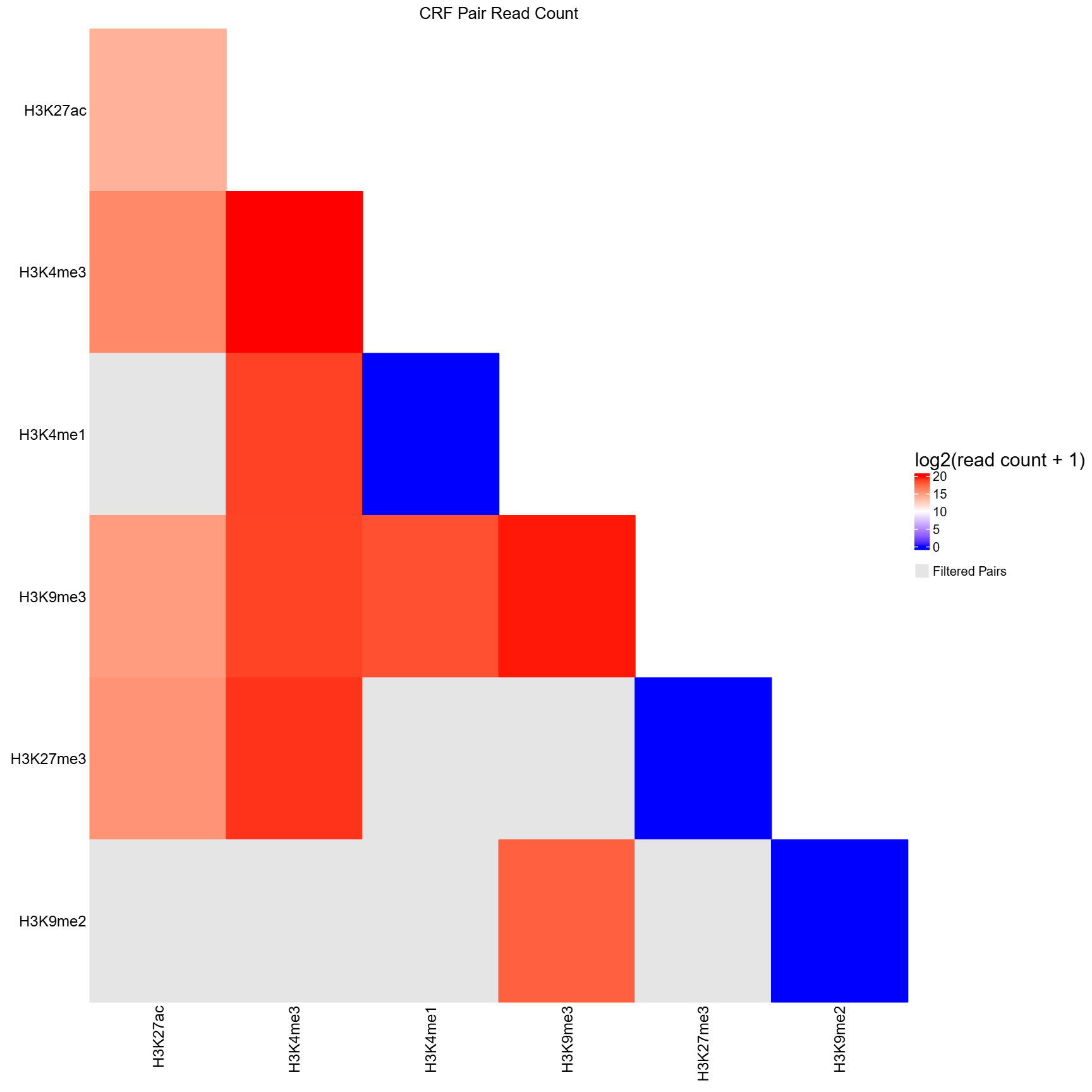
The qc_visualization() function performs read-level quality control visualization based on precomputed read count tables. It serves as the R-side visualization companion to the bash-based QC step (qc.sh), transforming pairwise read counts into a CRF-by-CRF heatmap for diagnostic inspection.

What this function does:

Unlike earlier integrated QC command, qc_visualization() does not compute read counts or apply filtering itself. Instead, it consumes two TSV files generated upstream.

Reads all_read_count.tsv and filtered_read_count.tsv, both containing CRF pair names (pair) and corresponding read counts (read_count).
Converts the pairwise table into a symmetric CRF-by-CRF matrix, filling only the lower triangle.
Marks CRF pairs that fail QC (i.e., not present in the filtered table) as NA, which are displayed in grey in the heatmap.
Applies a log2(read count + 1) transformation to stabilize dynamic range.
Generates a publication-quality PDF heatmap summarizing sequencing depth across all CRF pairs.
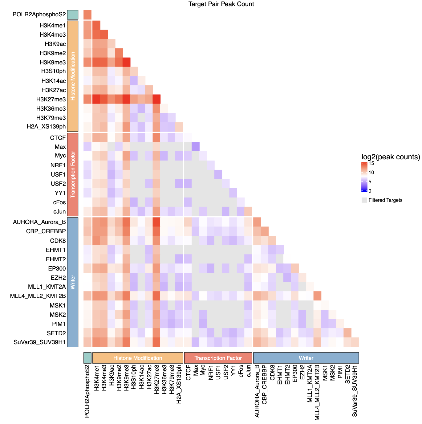
Optionally annotates CRFs by biological categories (e.g., histone marks, TFs) using a user-provided grouping CSV.

Parameter	Type	Default	Description	Example
`all_read_count_path`	character	—	Path to `all_read_count.tsv` containing all CRF pairs and their read counts	`“qc/all_read_count.tsv”`
`filtered_read_count_path`	character	—	Path to `filtered_read_count.tsv` containing CRF pairs that pass QC	`“qc/filtered_read_count.tsv”`
`out_dir`	character	`“.”`	Output directory for the heatmap PDF	`out_dir = “./qc”`
`split_pair_by`	character	`“-”`	Delimiter used to split CRF pair names into individual CRFs	`split_pair_by = “_“`
`group_csv`	character	`NULL`	Optional CSV defining CRF groupings for heatmap annotation	`“crf_groups.csv”`
`crf_col`	character	`“crf”`	Column name in `group_csv` specifying CRF identifiers	`crf_col = “CRF”`
`category_col`	character	`“category”`	Column name in `group_csv` specifying CRF categories	`category_col = “group”`

Output Files

The function generates the following output files in the specified out_dir:

Peak count heatmap - qc_heatmap.pdf (if plot = TRUE)
- PDF visualization of log2-transformed read counts for CRF-CRF pairs
- Lower triangle matrix showing read counts between CRF pairs
- Filtered (non-significant) pairs displayed in grey
- If group_csv provided, includes categorical annotations with colored blocks

Heatmap of log2-transformed read counts (log2(read count + 1)) for CRF–CRF pairs in the test dataset. Grey cells indicate CRF pairs without valid read counts, including both pairs removed during quality control and pairs that were not present in the dataset. This reflects the selection of the test data, which does not contain all possible 2 × 2 CRF combinations.

Heatmap of log2-transformed peak counts for CRF–CRF target pairs in the full dataset (36 CFRs). CRFs are grouped by functional class, including histone modifications, transcription factors, and writers. Grey cells indicate CRF pairs that were excluded by quality control filtering.

Example Usage

library(multiEpiCore)

# ===== General Usage =======
# Define QC directory
qc_dir <- "qc"

# Optional: Create grouping CSV
crfs <- c("H3K4me1", "H3K4me3", "H3K9ac", "H3K9me2", "H3K9me3", "H3K27ac", "H3K27me3", "H3K36me3")
categories <- c(rep("Active", 3), rep("Repressive", 3), rep("Other", 2))
group_df <- data.frame(crf = crfs, category = categories)
write.csv(group_df, file.path(qc_dir, "crf_groups.csv"), row.names = FALSE)

# Run QC with grouping
qc_visualization(
  all_read_count_path = file.path(qc_dir, "all_read_count.tsv"),
  filtered_read_count_path = file.path(qc_dir, "filtered_read_count.tsv"),
  out_dir = qc_dir,
  split_pair_by = "-",
  group_csv = file.path(qc_dir, "crf_groups.csv")
)

# ===== Test Data =======
bam_dirs <- list(
  "C1" = 'qc/C1',
  "C2" = 'qc/C2',
  "T1" = 'qc/T1',
  "T2" = 'qc/T2'
)

for (name in names(bam_dirs)) {
  qc_by_percentile(
    all_read_count_path = file.path(bam_dirs[[name]], "all_read_count.tsv"),
    filtered_read_count_path = file.path(bam_dirs[[name]], "filtered_read_count.tsv")
  )
}

2. (Optional) Fragment Length Analysis

The frag_decomposition() function analyzes fragment length distributions from BAM or BED files to characterize chromatin structure patterns.

What this function does:

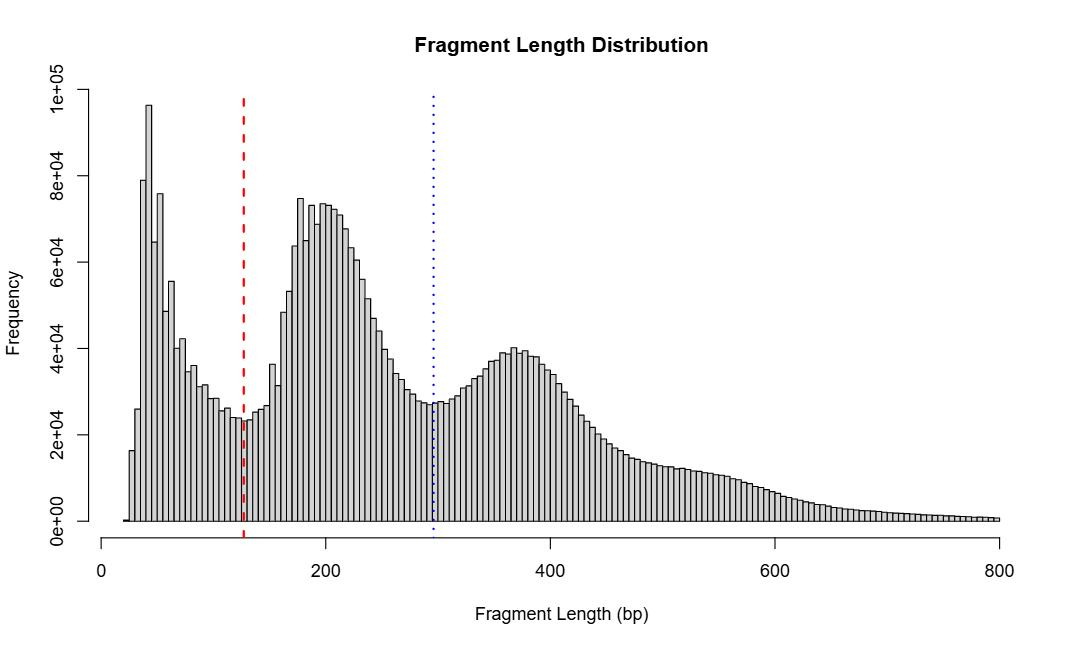
This function reads sequencing data files and extracts fragment lengths for all samples. It generates a combined histogram showing the overall fragment length distribution across all samples.

When detect_valley = TRUE, the function uses kernel density estimation to identify two valley positions in the distribution: the first valley (~150 bp) separates nucleosome-free regions from mononucleosome-bound fragments, and the second valley (~300 bp) separates mononucleosomes from dinucleosomes. These valleys serve as thresholds to classify each fragment into one of three categories: subnucleo (short fragments from open chromatin), monomer (single nucleosome), or dimer+ (multiple nucleosomes).

The function then calculates the count and percentage of fragments in each category for every sample, providing a quantitative assessment of chromatin accessibility. All results are saved as a histogram PDF and a TSV file containing per-sample decomposition statistics.

Parameters

Parameter	Type	Default	Description	Example
`file_path`	character vector	—	Vector of BAM or BED file paths to analyze for fragment length distribution	`file_path = c(“sample1.bam”, “sample2.bam”)`
`out_dir`	character	`“.”`	Output directory	`out_dir = “./frag_analysis”`
`detect_valley`	logical	`FALSE`	If TRUE, detects valley positions in the fragment length distribution to classify fragments into subnucleo, monomer, and dimer+ categories	`detect_valley = TRUE`
`dens_reso`	numeric	`2^15`	Resolution for kernel density estimation; higher values produce smoother curves	`dens_reso = 2^16`
`dens_kernel`	character	`“gaussian”`	Kernel type for density estimation (options: “gaussian”, “epanechnikov”, “rectangular”, “triangular”, “biweight”, “cosine”)	`dens_kernel = “epanechnikov”`
`valley1_range`	numeric vector	`c(73, 221)`	Range to search for the first valley (NFR/mononucleosome boundary)	`valley1_range = c(100, 180)`
`valley2_range`	numeric vector	`c(221, 368)`	Range to search for the second valley (mono/dinucleosome boundary)	`valley2_range = c(250, 350)`

Output Files

The function generates the following output files in the specified out_dir:

Fragment length histogram - fragment_distribution.pdf
- Shows the combined fragment length distribution across all samples
- If detect_valley = TRUE, includes red and blue vertical lines marking the two detected valley positions
- Visualizes the overall chromatin structure pattern

Fragment decomposition data - fragment_decomposition.tsv (only if detect_valley = TRUE)
- Per-sample statistics table with the following columns:
  - pair: Sample name (filename without extension)
  - total_count: Total number of fragments
  - subnucleo_count / subnucleo_pct: Count and percentage of fragments < valley1 (nucleosome-free regions)
  - monomer_count / monomer_pct: Count and percentage of fragments between valley1 and valley2 (mononucleosomes)
  - dimer_plus_count / dimer_plus_pct: Count and percentage of fragments ≥ valley2 (dinucleosomes and higher)

pair	total_count	subnucleo_count	subnucleo_pct
H3K27ac-H3K27ac	15198	6052	39.8210290827741
H3K27ac-H3K27me3	43569	9697	22.2566503706764
H3K27ac-H3K4me1	31754	6028	18.9834351577754
H3K27ac-H3K4me3	60573	11751	19.3997325541083
H3K27ac-H3K9me3	32173	7423	23.0721412364405
H3K27me3-H3K4me3	574643	127471	22.1826420925688
H3K4me1-H3K4me3	432292	86923	20.1074736520685
H3K4me1-H3K9me3	307657	65218	21.1982825029172
H3K4me3-H3K4me3	940240	191717	20.3902195184208
H3K4me3-H3K9me3	415540	98901	23.8005968137845
H3K9me2-H3K9me3	201788	49676	24.6179158324578
H3K9me3-H3K9me3	820666	178360	21.7335676145959

pair	monomer_count	monomer_pct	dimer_plus_count	dimer_plus_pct
H3K27ac-H3K27ac	4766	31.3593893933412	4380	28.8195815238847
H3K27ac-H3K27me3	20374	46.762606440359	13498	30.9807431889646
H3K27ac-H3K4me1	12538	39.4847893178812	13188	41.5317755243434
H3K27ac-H3K4me3	21792	35.9764251399138	27030	44.6238423059779
H3K27ac-H3K9me3	13164	40.9162962732726	11586	36.0115624902869
H3K27me3-H3K4me3	274641	47.7933255951956	172531	30.0240323122356
H3K4me1-H3K4me3	176829	40.9049901455498	168540	38.9875362023817
H3K4me1-H3K9me3	134247	43.6352821486266	108192	35.1664353484562
H3K4me3-H3K4me3	343196	36.500893388922	405327	43.1088870926572
H3K4me3-H3K9me3	178033	42.843769552871	138606	33.3556336333446
H3K9me2-H3K9me3	79756	39.5246496322873	72356	35.8574345352548
H3K9me3-H3K9me3	341684	41.634964772514	300622	36.63146761289

Example Usage

library(multiEpiCore)

# ===== Test Data =======
bam_dirs <- list(
  "C1" = 'bam/C1',
  "C2" = 'bam/C2',
  "T1" = 'bam/T1',
  "T2" = 'bam/T2'
)

for (name in names(bam_dirs)) {
  bam_dir <- bam_dirs[[name]]
  bam_paths <- list.files(path = bam_dir, pattern = "\\.bam$", recursive = TRUE, full.names = TRUE)
  frag_decomposition(
    file_paths = bam_paths, 
    out_dir = file.path("qc", name),
    detect_valley = TRUE
  )
}

QC Visualization

1. Read-Level QC (Visualization)

Output Files

Example Usage

2. (Optional) Fragment Length Analysis

Parameters

Output Files

Example Usage