1. Read-Level QC

The all_qc_with_plot() function performs quality control on BAM/BED files and generates a log2-transformed peak count heatmap for tag-tag pairs.

What this function does:

Performs quality control analysis on BAM or BED files
Calculates read counts and peak counts for all tag pairs
Filters samples based on read count percentiles
Generates a heatmap visualizing peak counts between tag pairs
Highlights filtered (non-significant) pairs in the heatmap
Supports optional tag grouping and categorical annotation
Saves QC summary files and visualization as outputs

Parameters

Parameter	Type	Required	Description	Example
`file_path`	character vector	Yes	Vector of BAM or BED file paths for QC and visualization	`file_path = c("sample1.bam", "sample2.bam")`
`filtered_path`	character vector	No (default: NULL)	Optional vector of file paths for filtered QC matrix	`filtered_path = c("filtered1.bam", "filtered2.bam")`
`filtered_percentile`	numeric	No (default: 0.25)	Numeric value between 0 and 1 to filter the lowest-read-count samples	`filtered_percentile = 0.25`
`output_path_dir`	character	No (default: NULL)	Directory to store output CSVs and PDF. If NULL, uses the directory of the first input file	`output_path_dir = "./results"`
`split_crf_by`	character	No (default: “-”)	Delimiter used to split tag pairs into individual TF names	`split_crf_by = "-"`
`save`	logical	No (default: TRUE)	If TRUE, writes CSV files and total reads summary	`save = TRUE`
`group_csv`	data frame	No (default: NULL)	Optional data frame defining tag groupings and categories for annotation	`group_csv = data.frame(tag = c("YY1", "cJun"), category = c("Group1", "Group2"))`
`tag_names`	character	No (default: “tag”)	Column name in `group_csv` for tag identifiers	`tag_names = "TF_name"`
`category_names`	character	No (default: “category”)	Column name in `group_csv` for group categories	`category_names = "TF_family"`
`target_pair_mapping_df`	data frame	No (default: NULL)	Optional data frame for renaming tag names in the heatmap matrix	`target_pair_mapping_df = NULL`

Output Files

The function generates the following output files in the specified output_path_dir:

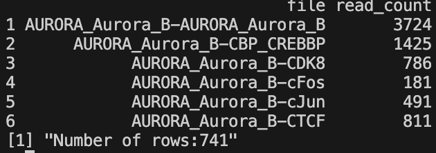
All read counts CSV - all_read_counts_bam.csv or all_read_counts_bed.csv
- Contains read counts for all input files
- Two columns: file name and read count
- Generated only if save = TRUE
- File extension depends on input file type (BAM or BED)
Filtered read counts CSV - filtered_read_counts_bam.csv or filtered_read_counts_bed.csv
- Contains read counts for files passing the percentile filter
- Excludes samples in the lowest percentile based on filtered_percentile parameter
- Two columns: file name and read count
- Generated only if save = TRUE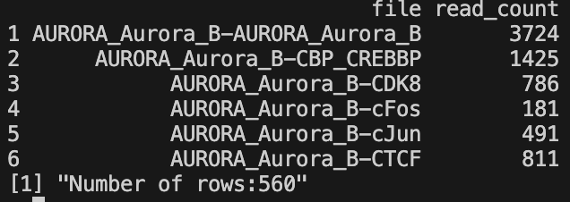
Total reads summary - total_reads.txt
- Text file containing total read count across all samples
- Single numeric value
- Generated only if save = TRUE
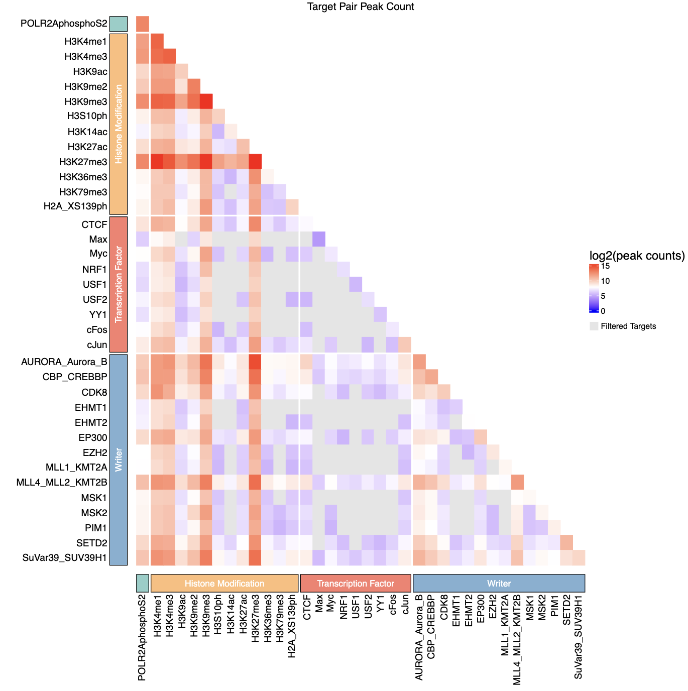
Peak count heatmap - AAA_test_qc_heatmap.pdf
- PDF visualization of log2-transformed peak counts for tag-tag pairs
- Lower triangle matrix showing peak counts between transcription factor pairs
- Filtered (non-significant) pairs displayed in grey
- Color scale: blue (low) → white (medium) → red (high)
- If group_csv provided, includes categorical annotations with colored blocks
- Dimensions: 12 × 12 inches

Example Usage

# bed file:
input_path <- "./dir_for_bed_files"
bed_files <- list.files(path = input_path, pattern = "\\.bed$", recursive = TRUE, full.names = TRUE)

# test csv
tags <- c("H3K4me1", "H3K4me3", "H3K9ac", "H3K9me2", "H3K9me3", "H3S10ph", "H3K14ac", "H3K27ac", "H3K27me3", "H3K36me3", "H3K79me3", "H2A_XS139ph", "POLR2AphosphoS2", "AURORA_Aurora_B", "CBP_CREBBP", "CDK8", "EHMT1", "EHMT2", "EP300", "EZH2", "MLL1_KMT2A", "MLL4_MLL2_KMT2B", "MSK1", "MSK2", "PIM1", "SETD2", "SuVar39_SUV39H1", "CTCF", "Max", "Myc", "NRF1", "USF1", "USF2", "YY1", "cFos", "cJun")

splits <- c(rep(1, 12), 2, rep(3, 14), rep(4, 9))

group_labels <- c("Histone Modification", "", "Writer", "Transcription Factor")
group <- group_labels[splits]

group_df <- data.frame(tag = tags, category = group)

library(epigenomeR)
all_qc_with_plot(file_path = bed_files, filtered_path = NULL, output_path_dir = "output/qc_heatmap", group_csv = group_df)

Notes

The function automatically detects whether input files are BAM or BED format based on file extensions.
The filtered_percentile parameter removes samples with the lowest read counts (e.g., 0.25 removes the bottom 25%).
If filtered_path is provided, it overrides the percentile-based filtering for determining significant pairs in the heatmap.
The heatmap displays only the lower triangle of the matrix, with filtered pairs shown in grey.
Peak counts are log2-transformed (log2(count + 1)) for visualization.
When group_csv is provided, tags are sorted by category and displayed with colored block annotations.
The function requires the following R packages: ComplexHeatmap, latex2exp, circlize, and grid.
All file paths in file_path and filtered_path must exist, or the function will fail.
If output_path_dir is NULL, outputs are saved to the directory containing the first input file.

2. Fragment Length Analysis

The frag_decomposition() function performs a complete fragment length analysis pipeline including quality control, valley detection, and visualization for nucleosome positioning analysis from BAM files.

What this function does:

Performs quality control filtering on BAM files based on coverage percentile
Computes fragment lengths from filtered paired-end BAM files
Detects two local minimum valleys for nucleosome fragment classification
Generates fragment length histograms with valley cutoff lines
Creates summary statistics report (valley positions, min/max fragment lengths)
Produces fragment decomposition data with percentages
Generates bar plots showing fragment distribution across samples

Parameters

Parameter	Type	Required	Description	Example
`file_path`	character vector	Yes	Paths to BAM files to analyze	`file_path = c("sample1.bam", "sample2.bam")`
`save_dir`	character	Yes	Directory path to save all output files and plots	`save_dir = "./fragment_analysis"`
`frag_decomp_file`	character	No	Path to generated fragment decomposition file (returned by function)	Auto-generated
`filtered_percentile`	numeric	No	Percentile threshold for quality control filtering (default: 0.25, removes bottom 25%)	`filtered_percentile = 0.25`
`dens_reso`	numeric	No	Resolution for kernel density estimation in valley detection (default: 2^15 = 32768)	`dens_reso = 2^15`
`target_pair_mapping_df`	data frame	No	Optional data frame for mapping sample names to display names (default: NULL)	`target_pair_mapping_df = df`
`density_kernel`	character	No	Kernel type for density estimation (default: “gaussian”)	`density_kernel = "gaussian"`
`valley1_range`	numeric vector	No	Search range for first valley in bp (default: c(73, 221))	`valley1_range = c(73, 221)`
`valley2_range`	numeric vector	No	Search range for second valley in bp (default: c(222, 368))	`valley2_range = c(222, 368)`

Output Files

The function generates the following output files in the specified save_dir:

Fragment length data - premerge_all-qc_frag_lens.RData
- Cached fragment length data from all filtered samples
- Numeric vector of fragment lengths
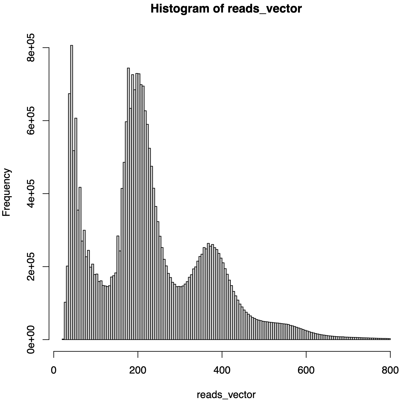
Initial histogram - premerge_frag_hist.pdf
- Fragment length distribution histogram without valley cutoffs
- Shows overall fragment length distribution
Summary report - summary_report.csv
- Contains key metrics:
  - local_min1: First valley position (bp)
  - local_min2: Second valley position (bp)
  - min_frag_len: Minimum fragment length (bp)
  - max_frag_len: Maximum fragment length (bp)
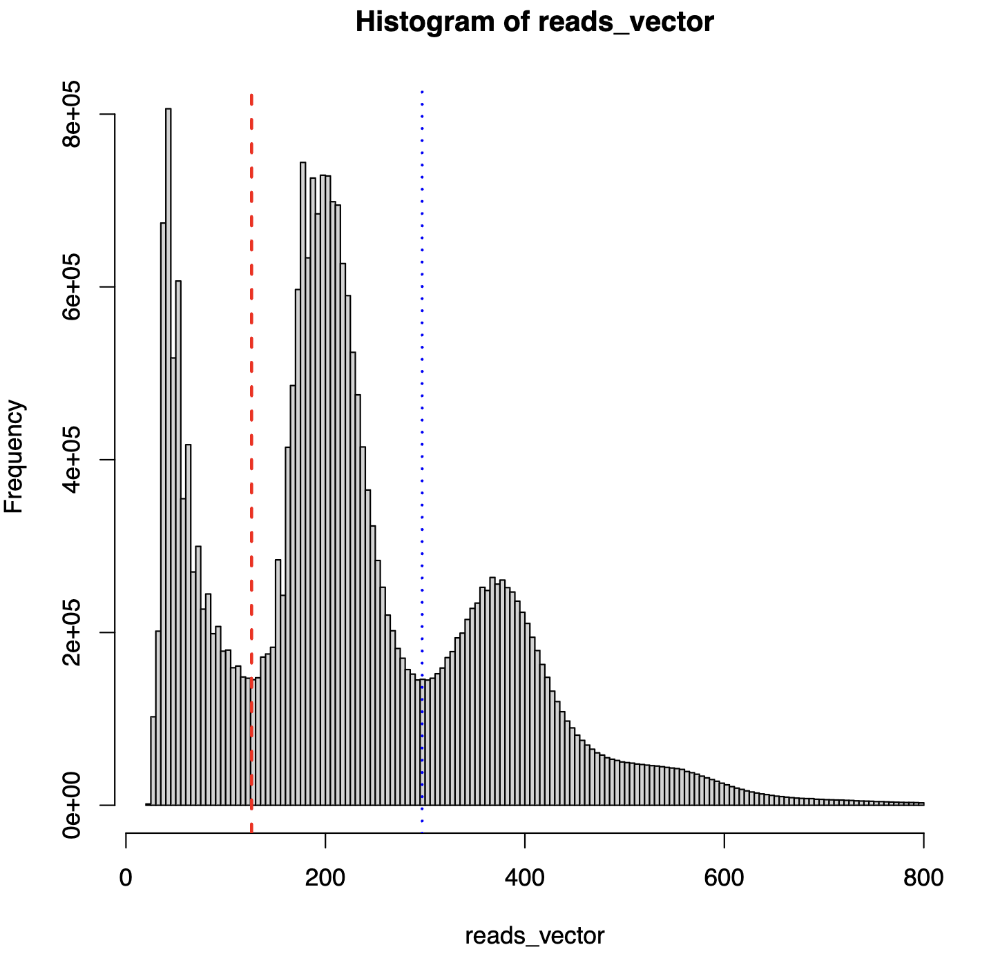
Histogram with cutoffs - premerge_frag_hist_with_cutoff.pdf
- Fragment length distribution with vertical lines at valley positions
- Used to visualize nucleosome fragment classification
Fragment decomposition data - *_frag_decomp_with_perc.tsv
- Per-sample fragment counts and percentages
- Classified by valley thresholds: subnucleo, monomer, dimer+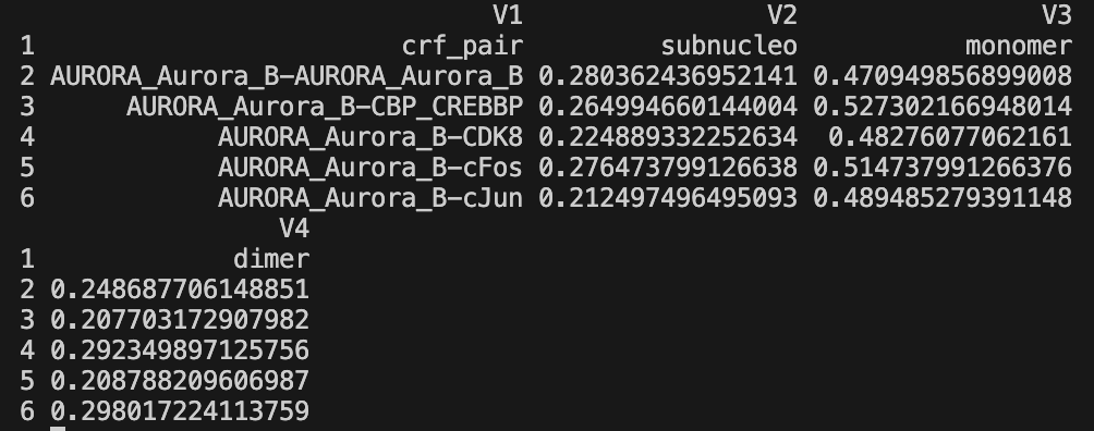
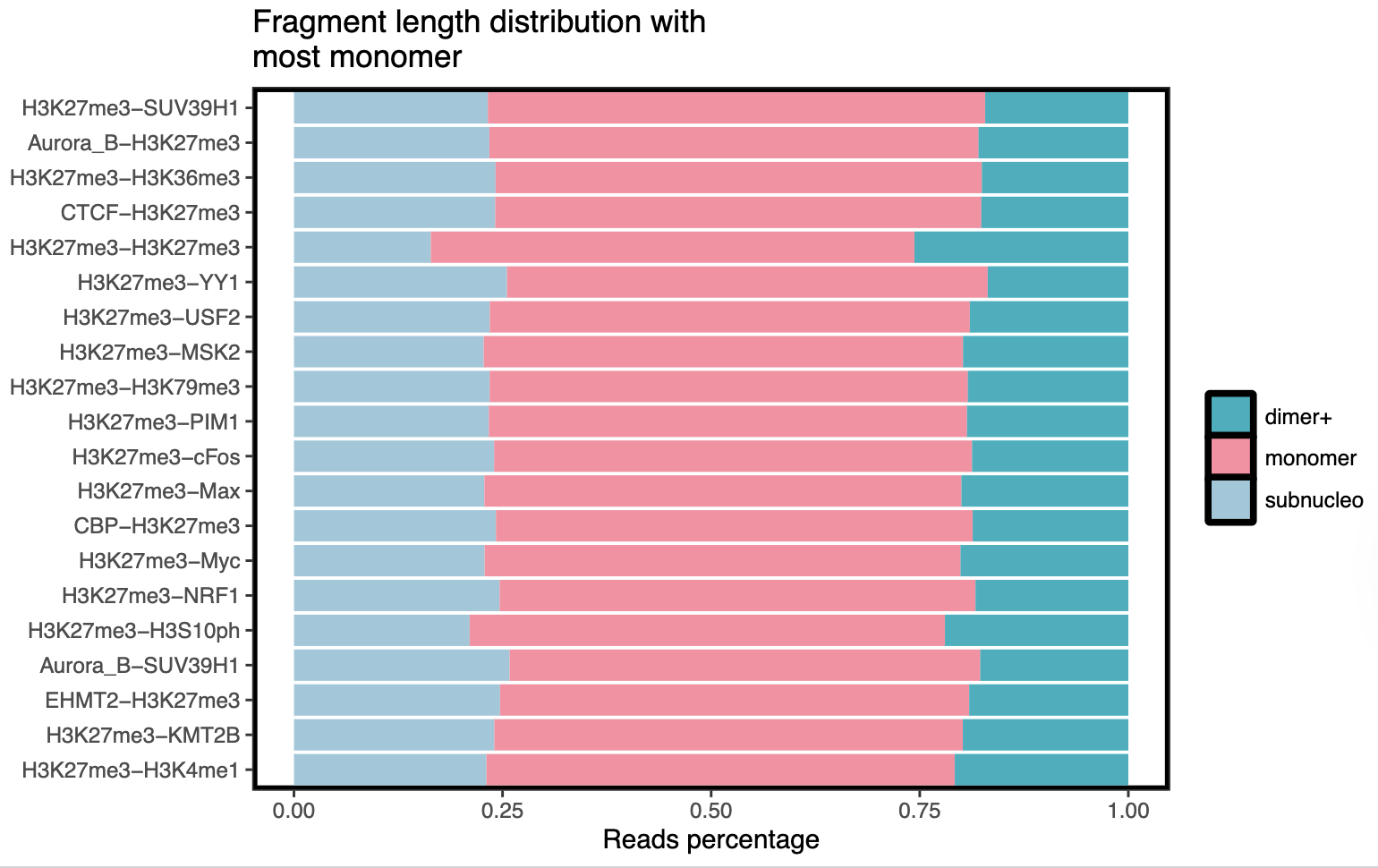
Bar plots - save_dir/barplots/*.pdf
- Visual representation of fragment distribution across samples
- Separate plots for different fragment categories

Example Usage

library(epigenomeR)
frag_decomposition(file_path = bam_files_vector, save_dir = "output/frag_decomposition")

3. Split bam files in bash

## Use in bash
## change with your length of scen_list
#SBATCH --array=0-1

module load samtools

# setup (change)
thres_name="valley-V-qc"
scen_list=( "T" "V" ) # input dir name
scen_simple_name_list=( "T" "V" ) # output name
target_list=( "IgG_control" "H3K36me3" "H3K4me1"... )
load_root_dir="./data_align" # directory path for scen_list
save_root_raw_dir="output/frag_decomposition/split_bam"

# main function
run_frag_decomposition() {
    scen=${scen_list[${SLURM_ARRAY_TASK_ID}]}
    scen_simple_name=${scen_simple_name_list[${SLURM_ARRAY_TASK_ID}]}

    save_root_dir=${save_root_raw_dir}/${thres_name}
    mkdir -p "${save_root_dir}"

    load_dir=${load_root_dir}/${scen}
    mixed_dir=${save_root_dir}/${scen_simple_name}_mixed
    subneucleo_dir=${save_root_dir}/${scen_simple_name}_sub
    mononeucleo_dir=${save_root_dir}/${scen_simple_name}_mono
    dineucleo_dir=${save_root_dir}/${scen_simple_name}_di

    mkdir -p "${mixed_dir}" "${subneucleo_dir}" "${mononeucleo_dir}" "${dineucleo_dir}"
    cp -r ${load_dir}/* "${mixed_dir}/"

    for target_1 in "${target_list[@]}"; do
        for target_2 in "${target_list[@]}"; do
            if [ "${target_1}" \< "${target_2}" ] || [ "${target_1}" = "${target_2}" ]; then
                mixed_filename="${target_1}-${target_2}.bam"
                mixed_dir_filename=${load_dir}/${mixed_filename}

                if [[ ! -f "${mixed_dir_filename}" ]]; then
                    echo "Warning: ${mixed_dir_filename} not found, skip."
                    continue
                fi
                samtools view -h ${mixed_dir_filename} | awk 'substr($0,1,1)=="@" || ($9>=24 && $9<=126) || ($9<=-24 && $9>=-126)' | samtools view -b > ${subneucleo_dir}/${mixed_filename}
                samtools view -h ${mixed_dir_filename} | awk 'substr($0,1,1)=="@" || ($9>=127 && $9<=297) || ($9<=-127 && $9>=-297)' | samtools view -b > ${mononeucleo_dir}/${mixed_filename}
                samtools view -h ${mixed_dir_filename} | awk 'substr($0,1,1)=="@" || ($9>=298 && $9<=800) || ($9<=-298 && $9>=-800)' | samtools view -b > ${dineucleo_dir}/${mixed_filename}
            fi
        done
    done
}

run_frag_decomposition

Quality Control

1. Read-Level QC

Parameters

Output Files

Example Usage

Notes

2. Fragment Length Analysis

Parameters

Output Files

Example Usage

3. Split bam files in bash